Your First Kaggle Experience
Your First Kaggle Experience
![]()
Introduction
Kaggle is an amazing community for aspiring data scientists and machine learning practitioners to come together to solve data science-related problems in a competition setting. Many statisticians and data scientists compete within a friendly community with a goal of producing the best models for predicting and analyzing datasets. Any company with a dataset and a problem to solve can benefit from Kagglers. Kaggle has not only provided a professional setting for data science projects, but has developed an environment for newcomers to learn and practice data science and machine learning skills.
This blog will serve as an introduction to the Kaggle platform and will give a brief walkthrough of the process of joining competitions, taking part in discussions, creating kernels, and progressing through the rankings.
Kaggle Progression System
Kaggle has a ranking system that helps data scientists track their progress and performance. Medals are awarded for certain activities that are completed. When a Kaggler earns enough medals to move up a tier in the progression system, they rank up!
Kaggle ranking can come from three different “categories of expertise”: Competitions, Kernels, and Discussion.
Each of the three categories has five ranks: Novice, Contributor, Expert, Master, and Grandmaster. The majority of Kaggle’s users are considered a “Novice”, which essentially means they have not interacted with the community and have not run any scripts or made any competition submissions. Every user above the Novice level has made submissions and has used datasets to make predictions and analysis.

A word to the wise, learn from everyone on Kaggle, especially the higher ranking individuals! One of the reasons behind Kaggle’s great success is its learning-friendly environment and the ease of learning new skills. Watching video tutorials about data science techniques is a great start, but there is nothing more valuable than reading through an experienced data scientist’s kernel and explanations, then using the skills you learned in your own models.
Discussion Board
The discussion board is a great place to ask questions, answer questions and interact with the community. There are always people posting answers to great questions that we can all learn from. There is also a “Getting Started” forum for the new Kagglers who want to learn the basics behind the Kaggle platform. Kaggle provides six unique forums in the discussion board where each forum has a different purpose.

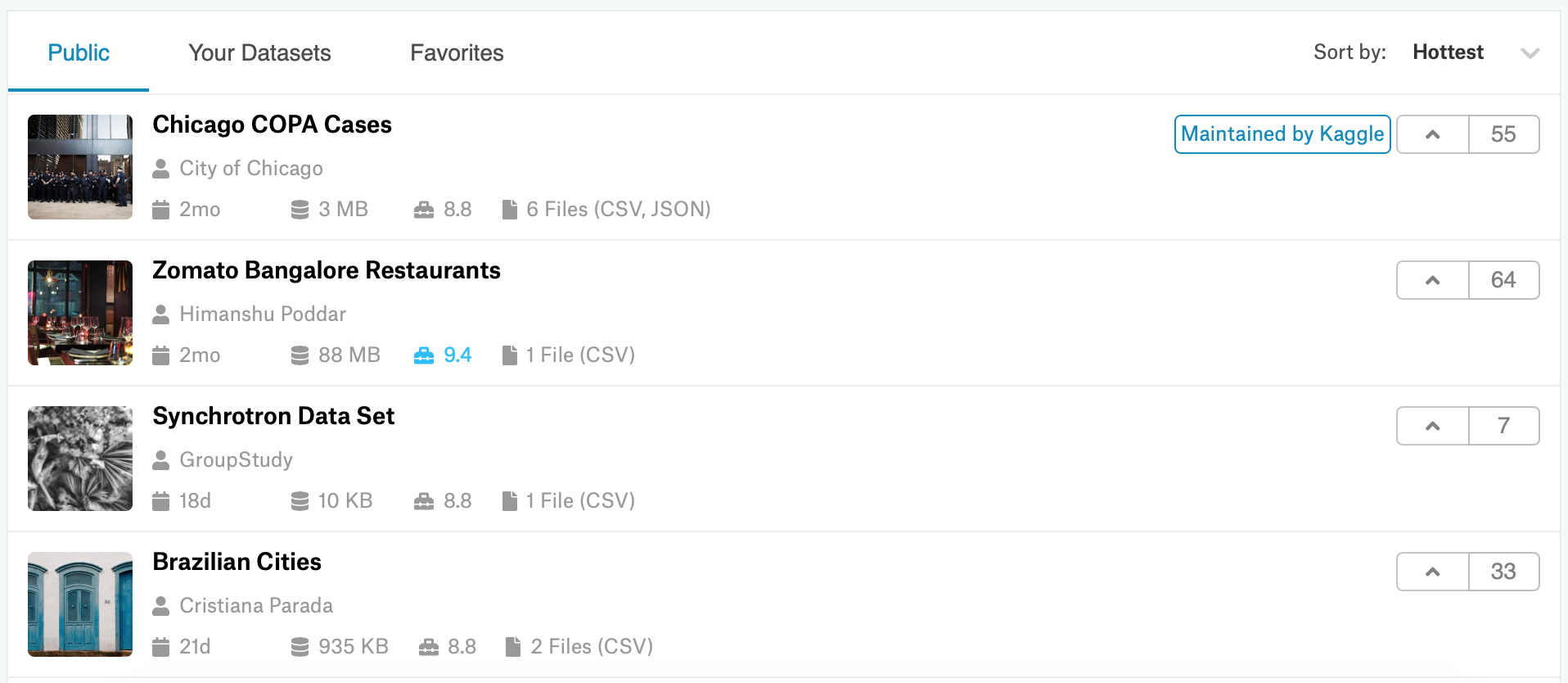
Datasets
You need data for any kind of data science project. Kaggle provides a vast amount of available datasets in its “Datasets” tab. As of the time of this blog, there are over 17,730 publicly available datasets. Datasets can be sorted by multiple filters to find exactly what you are looking for. Once you find the dataset that you want, you can simply click on it and click “Download” to download the data onto your machine.
Starting Your First Competition!
Under Kaggle’s “Competition” tab there are many competitions that you can join. This is just like the “Datasets” tab, where you can click on the competition and download the data for your models. There are a few competitions that are designed for beginners to enter and learn the basics of Kaggle and data science. One of the beginner friendly competitions is the famous MNSIT dataset, where we will create a model that will classify handwritten digits and produce predictions on test data. This blog post will use the MNIST dataset and will submit predictions to the competition as well. The first thing we need to do is look at our data and start thinking about building our model. To begin, we can start a new kernel.
Kernel
According to Kaggle’s documentation, Kernels are cloud computational environments that enable reproducible and collaborative analysis. Kernels allow a Kaggler to create and run code from within the browser without needing to download Python and the packages on their machine. One type of kernel that Kaggle provides is a notebook. If you are familiar with Jupyter Notebooks, then you are familiar with Kaggle’s notebooks because they are the same thing!
We will need to create our kernel, to do this, we can click “Create Kernel” and choose the “Notebook” option to do our analysis in Jupyter Notebook. Once the notebook opens, you will notice some prewritten code known as “starter code”. Starter code will import some common libraries and will print the directories within the data folder. For this blog, we will delete the starter code and write our imports by ourselves. In the first notebook cell, we will write all of the necessary imports for our project and we will print out everything that is in the “digit_data” folder that we downloaded.
import matplotlib.pyplot as plt
import seaborn as sns
import numpy as np
import pandas as pd
import os
print(os.listdir('digit_data'))
['test.csv', 'train.csv', 'sample_submission.csv']
The next step involves loading our data into the notebook. Notice that our data folder provides us with a train and test file. We can use pandas, a data analysis Python library, to read the CSV files into our train and test dataframes.
train = pd.read_csv('digit_data/train.csv')
test = pd.read_csv('digit_data/test.csv')
Once we have loaded in our data, we are going to want to get a sense of what the data is. To get a brief overview of what is in our dataset, we can use panda’s .head() method to print out the head, or top, of our dataset. We can set the number of rows that will be shown to 5.
train.head(5)
| label | pixel0 | pixel1 | pixel2 | pixel3 | pixel4 | pixel5 | pixel6 | pixel7 | pixel8 | |
|---|---|---|---|---|---|---|---|---|---|---|
| 0 | 1 | 0 | 0 | 0 | 0 | 0 | 0 | 0 | 0 | 0 |
| 1 | 0 | 0 | 0 | 0 | 0 | 0 | 0 | 0 | 0 | 0 |
| 2 | 1 | 0 | 0 | 0 | 0 | 0 | 0 | 0 | 0 | 0 |
| 3 | 4 | 0 | 0 | 0 | 0 | 0 | 0 | 0 | 0 | 0 |
| 4 | 0 | 0 | 0 | 0 | 0 | 0 | 0 | 0 | 0 | 0 |
5 rows × 785 columns
One of the first things we will have to do with our training data is split it into the inputs, or X (features) and the outputs (y). By looking at our data, we can see that the output (y) is the “label” column. This means our X data will be every column excpet the “label” column, and the y data will only be the “label” column. To seperate these we can use pandas’ .drop() method and give the name of the column we want to drop. To let pandas know that we want to drop a column, we will set “axis” to 1.
After splitting our training data, we can print the shapes of everything we have so far. After printing the shapes, we can also print the samples in both the test and training data. The shape of the training data will come out to be (42000, 784). This means that there are 42000 rows with 784 columns. Each row represents an individual digit in the data. Each column represents one pixel value for the image. Our images in the MNIST dataset should have a shape of 28x28 (28 x 28 = 784). Each image is flattened into one row.
x_train = train.drop('label', axis=1)
y_train = train['label'].astype('int32')

print('x_train shape: ', x_train.shape)
print('y_train shape: ', y_train.shape)
print('test shape: ', test.shape)
print('\nsamples in test: ', test.shape[0])
print('samples in train: ', x_train.shape[0])
x_train shape:  (42000, 784)
y_train shape:  (42000,)
test shape:  (28000, 784)

samples in test:  28000
samples in train:  42000
Let’s find out how many samples of each digit we have. For all we know, our data could be unbalanced and some digits may be represented more than others. This could cause our training to be hindered! To check how many samples of each digit we are training with, we can again use pandas and use the value_counts() method on the y training set.
print('Number of Examples Per Digit:\n', y_train.value_counts())
Number of Examples Per Digit:
 1    4684
7    4401
3    4351
9    4188
2    4177
6    4137
0    4132
4    4072
8    4063
5    3795
Name: label, dtype: int64
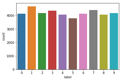
Another amazing high-level Python library that is used a lot in data science for visualization is Seaborn. Seaborn is a data visualization library that is heavily based on matplotlib, but is known to make more attractive graphics. Since we like attractiveness, we will work with Seaborn to visualize how many samples of each digit we have in our training set. After visualizing the balance within the data and after using pandas to view the exact amount of samples, we can confidently say that our data is very well balanced and that no digits are overrepresented.
sns.countplot(y_train)
<matplotlib.axes._subplots.AxesSubplot at 0x10b6eed30>
Each handwritten digit in the MNIST dataset has pixels that are an RGB value between 0-255. To normalize this range of values, we can divide each pixel value by 255. This will bring each pixel value closer together (within a 0-1 range) and keep things easier to learn from for our neural network. For example, an RGB value of 56 would then become .219, and an RGB value of 230 would become .901.
We can then reshape the values in both x_train and the test set. We will want to reshape them such that the number of samples comes first, then as mentioned earlier, each digit has the dimensions (28x28x1) or 28 rows, 28 columns and 1 color channel because the images are not colored.
x_train /= 255.0
test /= 255.0

x_train = x_train.values.reshape(x_train.shape[0], 28, 28, 1)
test = test.values.reshape(test.shape[0], 28, 28, 1)
Now we can print the final shape of the training and testing data.
print('x_train shape: ', x_train.shape)
print('y_train shape: ', y_train.shape)
print('test shape: ', test.shape)
x_train shape:  (42000, 28, 28, 1)
y_train shape:  (42000,)
test shape:  (28000, 28, 28, 1)
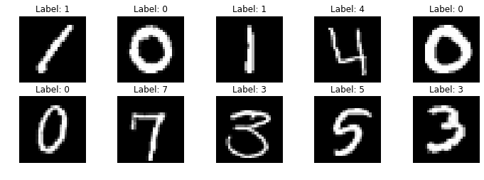
To view what the MNIST dataset contains, we can use pyplot from matplotlib and show eight images. The images will come from the training set (x_train) and above each image we can set the subplot title to be the corresponding output (y_train).
plt.figure(figsize=(12,10))

for img in range(10):
    plt.subplot(5, 5, img+1)
    plt.imshow(x_train[img].reshape((28, 28)), cmap='binary_r')
    plt.axis('off')
    plt.title('Label: ' + y_train[img].astype('str'))

plt.show()
Now we can start to create our model. To classify each digit we will use a convolutional neural network. Fortunately, Keras, a high-level Python neural network library, provides an easy and quick resource to build deep learning models. We will have to import Keras, the Sequential model and the necessary layers to use in our CNN.
import keras
from keras.models import Sequential
from keras.layers import Dense, Dropout, Flatten, Conv2D, MaxPooling2D
from keras.utils import to_categorical

from sklearn.model_selection import train_test_split
Using TensorFlow backend.
We can use Keras’ to_categorical() function to convert our class vector to a binary class matrix. Our classes in y_train are labeled as 1,2,3,4, etc. to_categorical() will create a matrix with as many columns as there are classes, and where a 1 indicates “yes” and a 0 indicates “no”. Keras’ documentation gives an intuitive example of this. You can view Keras’ docs here or see the example below:
# Consider an array of 5 labels out of a set of 3 classes {0, 1, 2}:
> labels
array([0, 2, 1, 2, 0])
# `to_categorical` converts this into a matrix with as many
# columns as there are classes. The number of rows
# stays the same.
> to_categorical(labels)
array([[ 1.,  0.,  0.],
       [ 0.,  0.,  1.],
       [ 0.,  1.,  0.],
       [ 0.,  0.,  1.],
       [ 1.,  0.,  0.]], dtype=float32)
Once this is done, our data is ready to be trained! We can split the data up into training and test sets and then start training our model.
y_train = to_categorical(y_train, 10)
x_train, x_test, y_train, y_test = train_test_split(x_train, y_train, test_size = 0.1, random_state=1)
Now we can create our CNN model, which thanks to Keras, is very easy. We will need to use 2-D convolutional layers, max-pooling layers and dense layers, which are fully connected layers. We will also use dropout and flatten. Flattening our data takes the resulting matrix from the convolutional and pooling layers and “flattens” it into one long vector of input data (column). Our output layer will use the softmax activation function with 10 output nodes (the number of classes in our data).
model = Sequential()
model.add(Conv2D(32, kernel_size=(3, 3), activation='relu', input_shape=(28,28,1)))
model.add(Conv2D(64, (3, 3), activation='relu'))

model.add(MaxPooling2D(pool_size=(2, 2)))

model.add(Dropout(0.25))

model.add(Conv2D(64, (3, 3), activation='relu'))
model.add(Conv2D(128, (3, 3), activation='relu'))

model.add(Dropout(0.25))

model.add(Flatten())
model.add(Dense(128, activation='relu'))
model.add(Dropout(0.5))
model.add(Dense(10, activation='softmax'))
Before we train the model, we must first define the loss function, the optimizer and the metrics by which we will evaluate our model.
model.compile(loss='categorical_crossentropy', optimizer='Adadelta', metrics=['accuracy'])
Now we can finally train our model! We will give the .fit() function our training data and have it run for 12 epochs or iterations.
model.fit(x_train, y_train, batch_size=128, epochs=12, verbose=1,
          validation_data=(x_test, y_test))
Train on 37800 samples, validate on 4200 samples
Epoch 1/12
37800/37800 [==============================] - 144s 4ms/step - loss: 0.3357 - acc: 0.8946 - val_loss: 0.1302 - val_acc: 0.9610
Epoch 2/12
37800/37800 [==============================] - 154s 4ms/step - loss: 0.0894 - acc: 0.9738 - val_loss: 0.0518 - val_acc: 0.9848
Epoch 3/12
37800/37800 [==============================] - 145s 4ms/step - loss: 0.0623 - acc: 0.9818 - val_loss: 0.0398 - val_acc: 0.9879
Epoch 4/12
37800/37800 [==============================] - 142s 4ms/step - loss: 0.0481 - acc: 0.9858 - val_loss: 0.0426 - val_acc: 0.9860
Epoch 5/12
37800/37800 [==============================] - 145s 4ms/step - loss: 0.0398 - acc: 0.9872 - val_loss: 0.0358 - val_acc: 0.9898
Epoch 6/12
37800/37800 [==============================] - 134s 4ms/step - loss: 0.0350 - acc: 0.9891 - val_loss: 0.0305 - val_acc: 0.9907
Epoch 7/12
37800/37800 [==============================] - 144s 4ms/step - loss: 0.0302 - acc: 0.9911 - val_loss: 0.0275 - val_acc: 0.9917
Epoch 8/12
37800/37800 [==============================] - 133s 4ms/step - loss: 0.0269 - acc: 0.9918 - val_loss: 0.0292 - val_acc: 0.9910
Epoch 9/12
37800/37800 [==============================] - 140s 4ms/step - loss: 0.0225 - acc: 0.9929 - val_loss: 0.0400 - val_acc: 0.9886
Epoch 10/12
37800/37800 [==============================] - 132s 3ms/step - loss: 0.0215 - acc: 0.9933 - val_loss: 0.0330 - val_acc: 0.9914
Epoch 11/12
37800/37800 [==============================] - 133s 4ms/step - loss: 0.0191 - acc: 0.9938 - val_loss: 0.0304 - val_acc: 0.9910
Epoch 12/12
37800/37800 [==============================] - 155s 4ms/step - loss: 0.0183 - acc: 0.9943 - val_loss: 0.0314 - val_acc: 0.9921


<keras.callbacks.History at 0x1a30906ac8>
It looks like our model did a decent job! We can evaluate the model and get its loss and accuracy for both the training and test sets. Once we receive the loss and accuracy we can print it out and round them for simplicity.
loss, accuracy = model.evaluate(x_test, y_test, verbose=0)
train_stat = model.evaluate(x_train, y_train, verbose=0)

print('Train Loss:     ', round(train_stat[0], 5))
print('Train Accuracy: ', round(train_stat[1]*100, 4), '%')
print('Test Loss:      ', round(loss, 5))
print('Test Accuracy:  ', round(accuracy*100, 4), '%')
Train Loss:      0.00551
Train Accuracy:  99.8413 %
Test Loss:       0.03136
Test Accuracy:   99.2143 %
Since our model is trained and has proven to be pretty accurate, we can start to make predictions. We will use Keras’ .predict() method to predict the outputs to each digit in the x_test data.
predictions = model.predict(x_test)
Since we are creating a kernel in Kaggle for a competition, we will need to create a new CSV file containing our predictions. This file will be our submission to the competition and once it is created, we are done the competition!
results = np.argmax(predictions, axis = 1)

results = pd.Series(results, name="Label")

submission = pd.concat([pd.Series(range(1,28001),name = "ImageId"),results],axis = 1)

submission.to_csv("submission.csv", index=False)
Conclusion
Kaggler provides a great platform to learn and apply the knowledge and skills you have gained to real competitions and datasets. There are a numerous amount of datasets to choose from and every competition involves a very friendly community that is there to help you. I would recommend signing up for Kaggle and trying it out!